| Game | n | Min | Median | Mean | Max |
|---|---|---|---|---|---|
| No limit | 41 | 0 | 2 | 15.6 | 100 |
| Capped | 42 | 0 | 2 | 10.7 | 128 |
The St Petersburg game: what our students actually paid
A classroom experiment, ACTL20004/ACTL90021 — Module 5 2026
1 The experiment
The design
- Two lectures on the same day, undergraduate and postgraduate. Splitting a single room was impractical, so each cohort answered both versions, with the order counterbalanced:
| Cohort | First question | Second question |
|---|---|---|
| UG | No limit | Capped at $1,048,576 |
| PG | Capped at $1,048,576 | No limit |
- Anonymous, through Poll Everywhere, with results hidden from the room while each poll was open — so nobody could see the emerging distribution before committing to a figure.
- Pooling across cohorts was meant to balance out order and cohort effects. Unequal response rates undermined that in practice (see Caveats).
What students were asked
- A fair coin is tossed until it first comes up heads. A first head on toss \(n\) pays \(\$2^n\). Students stated the most they would pay to play once.
- In the capped version the house pays at most \(2^{20} = \$1{,}048{,}576\) — the prize for a first head on toss 20 — and keeps paying that amount if the first head takes longer.
- Nothing about expectation, fairness or the paradox was mentioned. The exercise ran before any utility material was delivered.
2 The headline result
Willingness to pay
- The median willingness to pay was $2 in both games.
- Difference in medians: $0, with a 95% bootstrap confidence interval of [$-1, $3]; a Mann–Whitney test gives \(p = 0.74\).
- Removing the cap raises the expected payoff from $21 to infinity. It moved the median response by nothing at all.
What the Mann–Whitney test is asking
- The Mann–Whitney (Wilcoxon rank-sum) test compares two independent samples using only the ranks of the observations, so it needs no assumption of normality — useful here, where the responses are heavily skewed with a few very large values.
- \(H_0\): the two sets of responses come from the same distribution. Equivalently, a response drawn at random from the no limit game is as likely to fall above a response from the capped game as below it: \[H_0: \quad \Pr[X > Y] = \Pr[Y > X] = \tfrac12,\] where \(X\) is a response to the uncapped question and \(Y\) one to the capped question.
- \(H_1\): one game tends to elicit systematically higher answers than the other.
- With \(p = 0.74\) we have no evidence against \(H_0\) — consistent with the medians, the bootstrap interval and the two distribution functions.
- Careful: this is failure to reject, not proof of equality. See Caveats.
Responses side by side
Plot R code (result on the next slide):
brk <- c(-0.01, 1.5, 3, 6, 12, 24, 48, 96, 200)
lab <- c("$0-1", "$2", "$4", "$5-8", "$10-16",
         "$20-32", "$50-64", "$97+")
d2  <- transform(dat, bin = cut(wtp, brk, labels = lab))

ggplot(d2, aes(bin, fill = game)) +
  geom_bar(aes(y = after_stat(count) /
      tapply(after_stat(count), after_stat(fill),
             sum)[after_stat(fill)]), position = "dodge") +
  scale_y_continuous(labels = scales::percent) +
  scale_fill_manual(values = c("No limit" = "#0b4f8a",
                               "Capped"   = "#c1440e")) +
  labs(x = NULL, y = "share of responses", fill = NULL) +
  theme_minimal(base_size = 12) +
  theme(legend.position = "top",
        panel.grid.major.x = element_blank())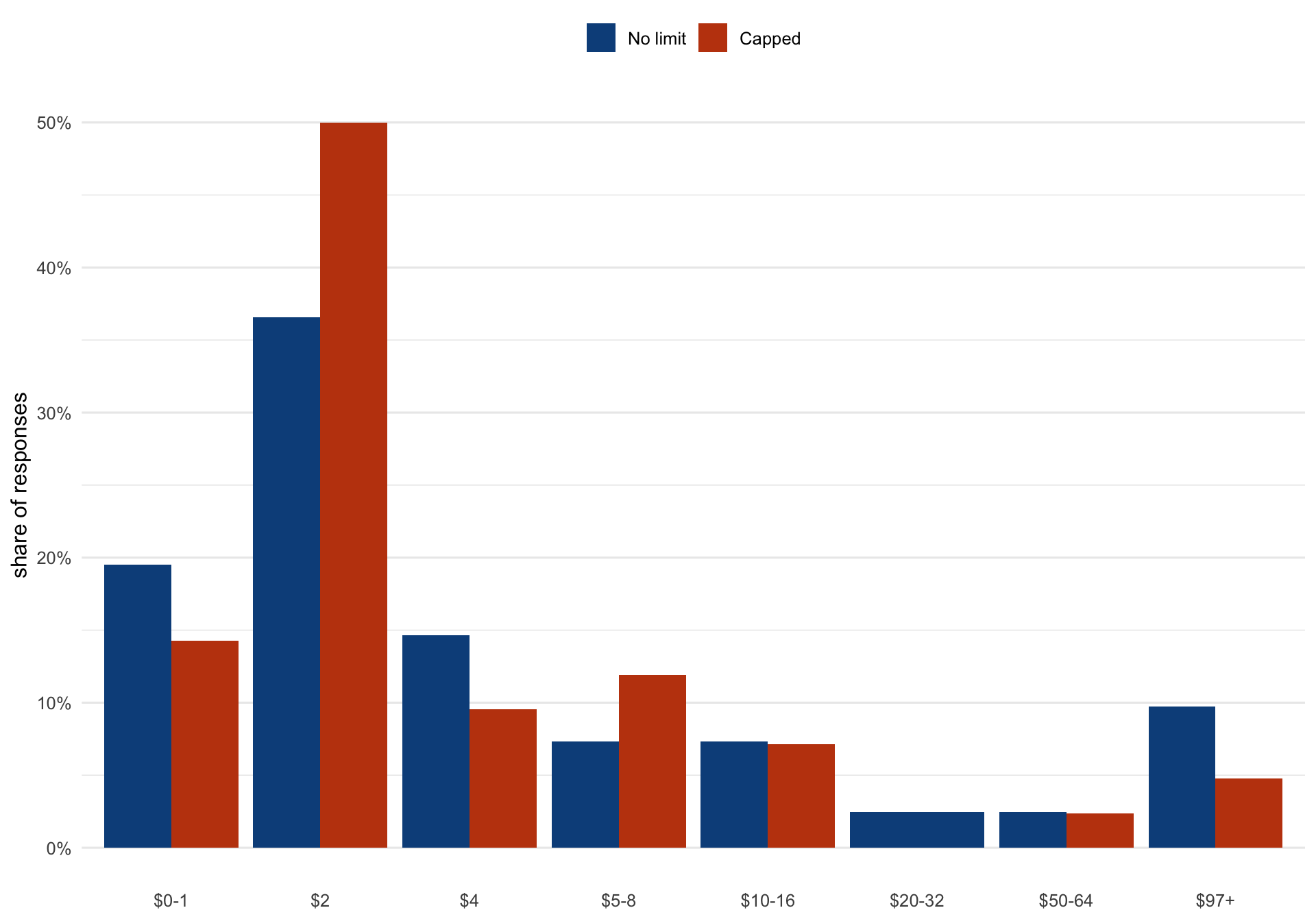
The two distributions coincide
Plot R code (result on the next slide):
ggplot(subset(dat, wtp > 0), aes(wtp, colour = game)) +
  stat_ecdf(linewidth = 1) +
  geom_vline(xintercept = fair_cap, linetype = "dashed",
             colour = "grey40") +
  annotate("text", x = fair_cap * 1.1, y = 0.15, hjust = 0,
           size = 3.4, colour = "grey30",
           label = paste0("fair value of\ncapped game = $",
                          fair_cap)) +
  scale_x_continuous(trans = "log2", breaks = pow2,
                     labels = paste0("$", pow2)) +
  scale_y_continuous(labels = scales::percent) +
  scale_colour_manual(values = c("No limit" = "#0b4f8a",
                                 "Capped"   = "#c1440e")) +
  labs(x = "willingness to pay (log scale)",
       y = "share paying at most this", colour = NULL) +
  theme_minimal(base_size = 12) +
  theme(legend.position = "top")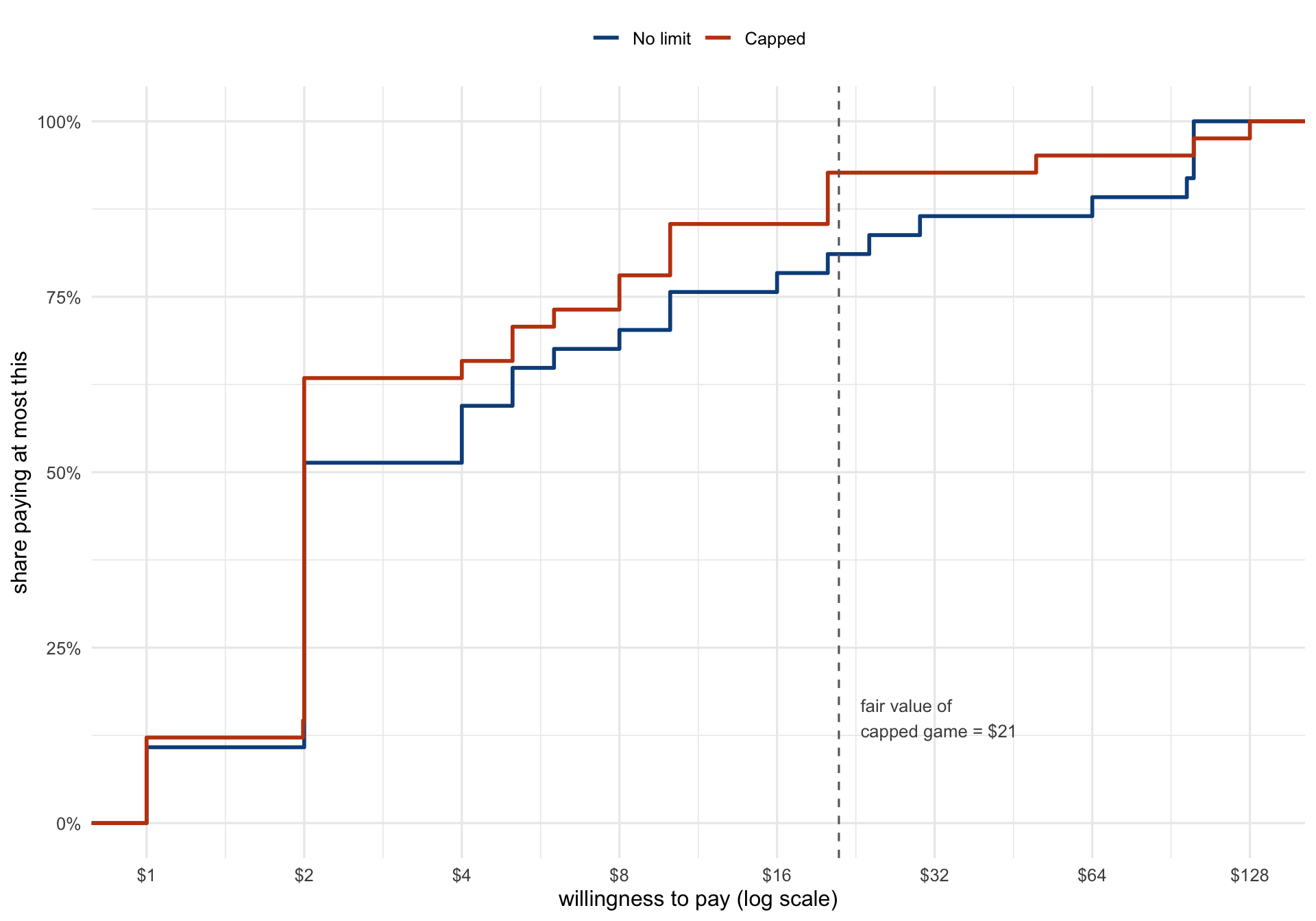
3 Why $2?
$2 is a structural answer, not a careless one
The obvious reading of the null result is that students simply ignore the tail. That is too harsh on them: $2 is a structural number, in two distinct senses.
- $2 is the guaranteed minimum payout. Pay it and you cannot lose money under any realisation of the game. It is the maximin answer.
- $2 is also the median and the mode of the payoff distribution, since \(\Pr(\text{payoff} = 2) = \tfrac12\) exactly.
The second point is the one that matters, because of the following invariance.
An invariance that explains the null
| Measure | No limit | Capped |
|---|---|---|
| Mean | \(\infty\) | $21 |
| Median | $2 | $2 |
| Mode | $2 | $2 |
- Truncation changes the mean from infinity to $21. It leaves the median and the mode at exactly $2, because half of all realisations end on the first toss regardless of the tail.
- So the answers are internally consistent: if you price the typical outcome rather than the average one, the cap genuinely is irrelevant.
- Utility theory tells us which functional of the payoff distribution to price — and the answer is neither the mean nor the mode.
4 What the free-text answers reveal
Jensen’s inequality, in the wild
Mean of this geometric distribution is 1, meaning the most willing to pay to get even is 2
- The student computed \(\mathbb{E}[N]\) and substituted it into the payoff function, evaluating \(2^{\mathbb{E}[N]}\) in place of \(\mathbb{E}[2^N]\).
- For a convex payoff these are not equal — here they differ by an infinite amount:
\[2^{\mathbb{E}[N]} = 2 \quad\text{but}\quad \mathbb{E}\!\left[2^{N}\right] = \sum_{n\ge1} 2^{-n}\,2^{n} = \infty.\]
- Jensen’s inequality, stated by a (forgetful) student!
The same cap, two statistics
2 - 0.5^20
- Submitted in the capped game: this student engaged seriously with the cap and adjusted their price downwards by about one part in a million, i.e. \(\approx 10^{-6}\).
- That is right if you are pricing the median, and wrong by an infinite margin if you are pricing the mean, where the same cap is the difference between $21 and infinity.
- One truncation, two risk measures, infinitely different conclusions — which is why the choice of risk measure is not a technicality.
The only tail pricer
Very very much, half to the maximum possible payout
- Roughly $524,288 — the only response anywhere near the tail.
- Notably submitted in the capped game: the cap supplied a finite anchor that made the thought expressible.
- A fourth student answered simply “Infinity” in the uncapped game, which is the only literally correct expected value in the dataset.
5 Two secondary findings
Risk aversion needs no comparison
- The capped game has an ordinary, finite, computable fair value of $21.
- Only 7% of students would pay more than that. That is, 93% declined a lottery offered at or below its expected value.
- This stands entirely on its own: no comparison between conditions, no counterbalancing, and none of the caveats below. If the experiment is repeated with limited time, the capped question alone delivers the Module 5 motivation.
The payoff ladder anchored the answers
- 65% of all numeric responses were exact powers of two, against only 17% at the round decimal figures one would otherwise expect people to reach for.
- The question displayed the prize schedule as $2, $4, $8, $16 — and students answered in the currency of that schedule.
- Less a flaw in the instrument than a demonstration that the presentation of a payoff schedule shapes the prices elicited against it.
6 Caveats
Caveats
- The counterbalancing did not balance. Response counts were 36 and 35 for UG, against 5 and 7 for PG. The pooled comparison is therefore the UG comparison with a small perturbation attached, and the cohort dimension is effectively lost.
- The surviving comparison is within-subject. UG students answered the capped question having already answered the uncapped one, so their second response may be anchored on their first. Given that the modal answer coincides with a structural constant of the game, anchoring seems unlikely to be doing much work — but it cannot be ruled out from these data.
- A null result is not evidence of equivalence. The confidence interval [$-1, $3] is tight enough to exclude any large shift, but with these sample sizes a modest one would not have been detected.
- PG numbers are indicative only. With 5 and 7 responses, the postgraduate cells should not be interpreted separately.
7 Where this leads
Where this leads
- The paradox is not that the expectation is infinite. It is that no reasonable person prices the expectation — and our own cohort supplies the evidence, in their own numbers, before the theory is introduced.
- Truncation is the standard textbook resolution, and our data suggest it resolves nothing behaviourally: the median is untouched because the median payoff is untouched.
- What does change behaviour is the shape of preferences over outcomes — which is exactly what utility theory supplies, and the transition into the rest of Module 5.