M8 Ruin Models
Topics in Insurance, Risk, and Finance
Introduction
Learning outcomes
- Understand the aggregate claim process and the cashflow process
- Compute and derive various probabilities of ruin
- Calculate the probability of ruin by simulations
- Know the adjustment coefficient and Lundberg’s inequality
- Show Lundberg’s inequality
- Derive bounds of the adjustment coefficient
Solvency
- Ruin theory is motivated by the practical issue of solvency.
- Solvency is a complicated topic.
- Simply speaking, an insurer is solvent if it has sufficient assets to meet its liabilities.
- This is a vague statement. How much capital is sufficient?
- In practice, regulators may require insurance companies to keep solvent over a period with a very high probability, say \(99\%\).
- This is where VaR appears as the regulatory risk measure.
Ruin
- Ruin theory is concerned with the level of an insurer’s surplus for a portfolio of insurance policies.
- We have done modelling insurance portfolio in a fixed period of time, e.g., the collective risk model: \[S=\sum_{i=1}^NX_i,\] where \(N\) is a random number.
- We will study the case when the number of claims evolves over time.
Ruin
We will study some surplus models consisting of three parts: initial surplus, premium, and claim payouts.
For simplicity, if the insurer’s surplus falls below zero, we say that ruin occurs.
We will mainly focus on the question:
Simple ruin models
Simple ruin models
- We first look at some simple examples of ruin models.
- These models are not standard in the actuarial literature.
- They can however serve as a good starting point since no prerequisite is required for these models.
- They do appear in actuarial exams!
Simple ruin model I
An insurance company has a portfolio of two-year policies. Aggregate annual claims from the portfolio follow an exponential distribution with mean 10 (independently from year to year). Annual premiums of 15 are payable at the start of each year. The insurer checks for ruin only at the end of each year. The insurer starts with no capital. Calculate the probability that the insurer is not ruined by the end of the second year.
Simple ruin model I
Simple ruin model II
An insurer insures a single building. The probability of a claim on a given day is \(p\) independently from day to day. Premiums of 1 unit are payable on a daily basis at the start of each day. The claim size is independent of the time of the claim and follows an exponential distribution with mean \(1/\lambda\). The insurer has a surplus of \(U\) at time zero.
Derive an expression for the probability that the first claim results in the ruin of the insurer.
Simple ruin model II
Simple ruin model III
[This is modified from question 9 of 2019 April CM2A exam]
An insurer offers a policy to actuarial students. The policy pays 500 when a student passes an exam. Students pay a premium 50 for each exam they take. Ruin happens if the surplus of the insurer is strictly less than 0.
There are two exam sessions each year, in April and October. Premiums are paid in the month of the exam. Exam results are published immediately after the exam.
The insurer has issued three policies on 1 January 2019 to students who are close to qualifying. The insurer assumes that each student has a \(25\%\) chance of qualifying in each future exam session. The insurer’s initial assets are 750.
Simple ruin model III
- Calculate the insurer’s assets after the April 2019 premiums are received.
- Calculate the probability of ruin when the April 2019 exam results are released.
Simple ruin model III
Assuming that no students qualified in April 2019:
- Calculate the insurer’s assets after the October 2019 premiums are received.
- Calculate the probability of ruin when the October 2019 exam results are released.
Simple ruin model III
Assuming that one student qualified in April 2019:
- Calculate the insurer’s assets after the October 2019 premiums are received.
- Calculate the probability of ruin when the October 2019 exam results are released.
Simple ruin model III
- Calculate the overall probability of ruin before the end of the year
- Explain the impact on the probability of ruin if the insurer issues more policies on the same terms.
Classical risk process
Counting process
A process \(N(t)\) is said to be a counting process, if
- \(N(0)=0\)
- \(N(t)\) takes non-negative integer values
- If \(s < t\), then \(N(s) \leq N(t)\), i.e., \(N(t)\) is non-decreasing in \(t\).
- For \(s < t\), \(N(t)- N(s)\) represents the number of events occurring in the time interval \((s, t]\).
Example: counting process
Consider \(n\) people aged \(x\) at time 0. Let \(N(t)\) be the number of deaths that occurred by time \(t\). Assume that the events of death are independent. Specify the distribution of \(N(t+h)-N(t)\) given \(N(t)\).
Poisson Process
A process \(N(t)\) with \(N(0)=0\) is a Poisson process with \(\lambda>0\) if the increment process has the following property: \[N(t+h)-N(t)\sim Poisson(\lambda h),\] for all \(t>0\), \(h>0\) and each history of \(N(s)\), \(s\le t\). As a result, we have the following two properties of a Poisson process:
- Independence: \(N(t)\) has independent increments, i.e., for \(0 \leq t_1 < t_2< \dots< t_{n-1} < t_n\), increments \(N(t_1),N(t_2)- N(t_1), \dots, N(t_n) - N(t_{n-1})\) are independent.
- Stationarity: \(N(t)\) has stationary increments, i.e. the distribution of \(N(t + h)- N(t)\) does not depend on \(t\), but depends on \(h\).
Poisson process
A process \(N(t)\) is a Poisson process with \(\lambda>0\) if
\(N(0)=0\)
Independence: \(N(t)\) has independent increments, i.e., for \(0 \leq t_1 < t_2< \dots< t_{n-1} < t_n\), increments \(N(t_1),N(t_2)- N(t_1), \dots, N(t_n) - N(t_{n-1})\) are independent.
Stationarity: \(N(t)\) has stationary increments, i.e. the distribution of \(N(t + h)- N(t)\) does not depend on \(t\), but depends on \(h\).
-
Over an infinitesimal time interval \((t, t + h]\).
\[\begin{align*} P(N(t+h)-N(t)=0)&=1-\lambda h+o(h),\\ P(N(t+h)-N(t)=1)&=\lambda h+o(h),\\ P(N(t+h)-N(t)\geq 2)&=o(h). \end{align*}\]
Here \(o(h)\) is a function such that \(o(h)/h\rightarrow 0\) as \(h\rightarrow 0\).
Poisson process
Let \(T_1,\dots,T_n\) be iid exponential random variables with mean \(1/\lambda\), representing the waiting times of successive claims. Let \(W_n =\sum_{i=1}^nT_i\) be the occurrence time of the \(n\)-th claim. Define \[N(t) = \max\{n:W_n\le t\}.\] Then \(N(t)\), \(t\ge 0\), is a Poisson process with parameter \(\lambda\).
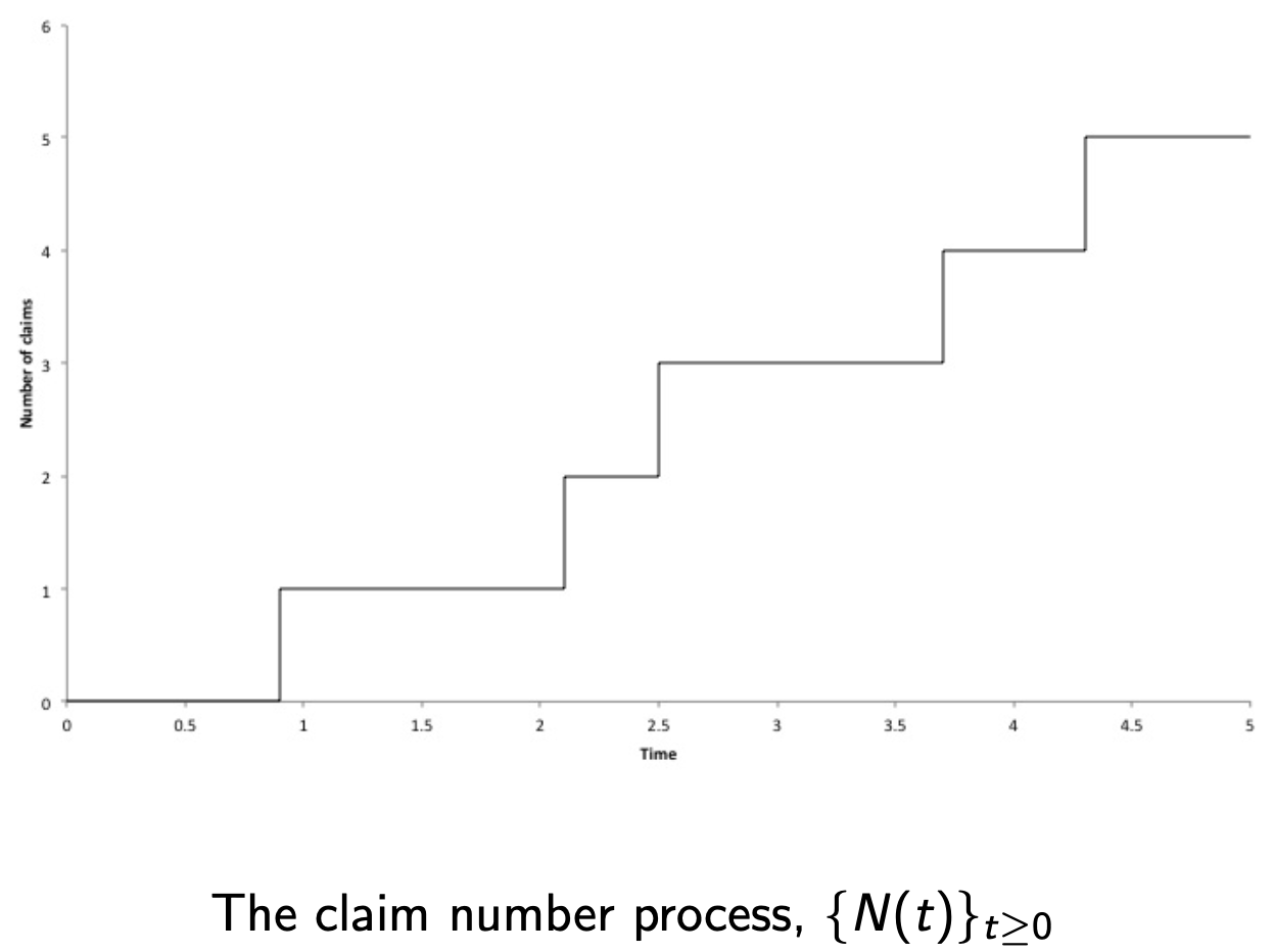
Example of a claim number process
Question: Can the size of jump be 2? How to run such a simulation?
Aggregate claims process
Consider an insurance company with the following loss portfolio over time interval \([0,t]\) for all \(t\geq 0\):
- \(N(t)\): number of claims up to time \(t\)
- \(X_i\): non-negative amount of the \(i\)-th claim, \(i=1,2,3,\dots\)
- \(X_1,X_2,\dots\) are iid
- \(\{N(t)\}\) and \(\{X_i\}\) are independent
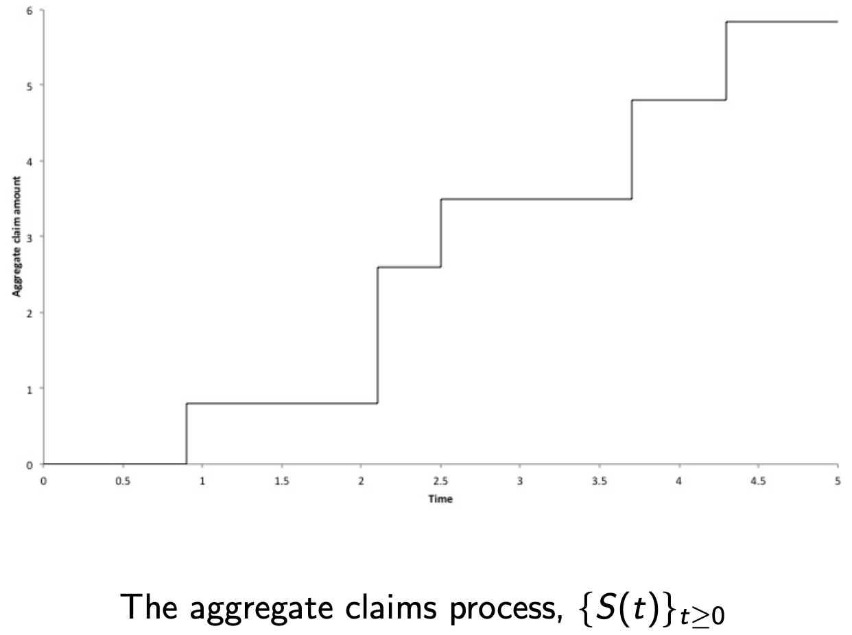
- \(S(t)\): the aggregate claims up to time \(t\), that is, \[S(t)=\sum_{i=1}^{N(t)}X_i\] with \(S(t)=0\) if \(N(t)=0\).
- \(S(t)\) is referred to as the aggregate claims process.
- If \(N(t)\) is a Poisson process, \(S(t)\) is a compound Poisson process.
Properties of compound Poisson processes
Notations:
- \(X_i\sim F\) with density \(f\) such that \(F(0)=0\) (i.e., \(X_i\), \(i=1,2,3,\dots\), are positive almost surely).
- \(m_k=\E(X_i^k)\), \(k=1,2,3,\dots\)
- \(M_{X}(r)=\E(\exp(rX_i))\)
We have
- \(\E(S(t))=\lambda t m_1\)
- \(\var(S(t))=\lambda t m_2\)
- \(M_{S(t)}(r)=\exp(\lambda t(M_X(r)-1))\)
Q: Can you derive these formulas?
Surplus claims process I
We make the following assumptions:
- The insurer has an initial surplus \(u\ge 0\).
- The premium income is received continuously by the insurer at a constant rate per unit of time, denoted by \(c>0\): the total premium received over the time interval \([0,t]\) is \(ct\).
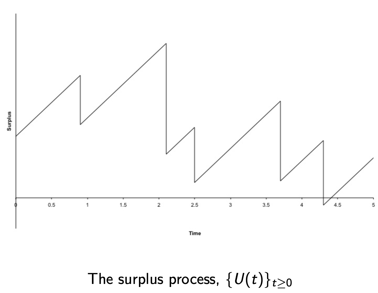
- The surplus claims process is defined as \[U(t)=u+ct-S(t), t\geq 0.\] Here, \(U(t)\) denotes the insurer’s capital at time \(t\).
- If \(S(t)\) is a compound Poisson process, we have the classical risk process.
Surplus claims process II
Note that
- Since \(u\) and \(c\) are deterministic, the only random part of \(U(t)\) comes from \(S(t)\).
- We need the initial surplus \(U(0)=u\) since premiums may not be sufficient to cover the claims.
Limitations:
- We ignore the expenses associated with the claim payments and interests possibly generated by the surplus.
- The claims are assumed to be paid out immediately.
- Reinsurance is also ignored (will be discussed later).
Despite these limitations, the model can still provide insights into an insurer’s operations.
Example of a aggregate claim process
Example of a surplus process
Ruin probability I
The state that \(U(t)<0\) for some \(t\) is called ruin.
- Ruin can be thought as insolvency.
- Denote the first time of ruin by \(T\), defined as, \[T=\min\{t> 0: U(t)<0\},\] with \(T=\infty\) if \(U(t)\geq 0\) for all \(t>0\).
Ruin probability II
- The continuous-time ultimate ruin probability is defined as \[\psi(u)=P(T<\infty).\]
- The continuous-time ruin probability in finite time is defined as \[\psi(u,t)=P(T<t).\]
Simple relations:
- \(\lim_{t\rightarrow \infty}\psi(u,t)=\psi(u)\)
- \(\psi(u,t)\le \psi(u)\)
Example: Normal approximation
Assume that \(N(t)\) is a Poisson process with parameter \(30\), the individual claim amount distribution is lognormal with parameters \(\mu=3\) and \(\sigma^2=1.1\), \(c=1200\), and \(u=1000\). Find \(P(U(2)<0)\) by assuming that \(S(t)\) is approximately normal.
Ruin probabilities against \(t\)
For \(0<t_1\le t_2<\infty\), and \(u\ge 0\), \[\psi(u,t_1)\le \psi(u,t_2)\le \psi(u).\] This is clear as \[\{T<t_1\}\subseteq \{T<t_2\}\subseteq \{T<\infty\}.\] Hence \(\psi(u,t)\) is an increasing function of \(t\).
Ruin probabilities against \(u\)
For \(0\le u_1\le u_2\), \[\psi(u_1)\ge \psi(u_2).\] This is because \[\psi(u)=\p(u+ct-S(t)<0~~ \mbox{for some}~~ t>0)\] and that \[\{u_2+ct-S(t)<0~~ \mbox{for some}~~ t>0\}\subseteq \{u_1+ct-S(t)<0~~ \mbox{for some}~~ t>0\}\] Hence, \(\psi(u)\) is a decreasing function of \(u\). Similarly, we have \[\psi(u_1,t)\ge \psi(u_2,t).\]
Ruin probabilities against \(\theta\)
- Probabilities \(\psi(u)\) and \(\psi(u,t)\) are both decreasing against \(\theta\).
- This is intuitively true as a larger \(\theta\) means more premium income.
- One can also prove this result using similar arguments for the previous result regarding ruin probabilities against \(u\).
Adjustment Coefficient and Lundberg’s inequality
Ultimate ruin probability
- Since it is impossible an insurer can survive for an infinite time, it is practical to consider ruin probabilities in finite time.
- However, ultimate ruin probabilities are more mathematically tractable and they can be used as the upper bounds for ruin probabilities in finite time.
Ruin probability for exponential claims
Example: exponential claims
Suppose \(X_1,X_2,\dots\) follow an exponential distribution \(F(x)=1-e^{-\alpha x}\) for \(x\ge 0\) and \(c=(1+\theta)\lambda m_1\). What is \(\psi(u)\)?
Lundberg’s inequality
- If \(c=(1+\theta)\lambda m_1\), the above equation reduces to \[ M_X(R)= 1+(1+\theta) m_1R,\] so that \(R\) is independent of the Poisson parameter \(\lambda\).
Additional comments
- For large initial surplus \(u\), the ultimate ruin probability is close to the upper bound. Hence, we have the approximation \[\psi(u)\approx \exp(-Ru),\] which is often used in actuarial literature.
- Clearly, the upper bound \(\exp(-Ru)\) decreases as \(R\) increases, where \(\exp(-Ru)\) is used as an approximation of \(\psi(u)\). Arguably, the ultimate ruin probability \(\psi(u)\) also decreases as \(R\) increases.
- By the second bullet point, we can regard the adjustment coefficient \(R\) as a (reverse) measure of risk for insurers: The larger \(R\) is, the less risk insurers face.
- \(e^{-R}\) can be regarded as the factor by which the ruin probability decreases given a unit increase in the initial surplus.
Example: exponential losses I
If the individual claims follow the exponential distribution \(F(x)=1-\exp(-\alpha x)\) for \(x\ge 0\), then \(M_X(r)=\alpha/(\alpha-r)\) for \(r< \alpha\). Find \(R\).
Example: exponential losses II
What if \(c=(1+\theta)\lambda m_1=(1+\theta)\lambda/\alpha\)? How is \(R\) affected by \(\theta\)?
Example: mixtures of exponential distributions
If the individual claims follow the distribution \[F(x)=1-0.5(\exp(-3 x)+\exp(-7 x)),\] for \(x\ge 0\), find \(R\) when \(\lambda=3\) and \(c=1\).
Proof of Lundberg’s inequality I
- \(\psi_n(u)\): probability that ruin happens before or at \(n\)-th claim, \(n=1,2,\dots\)
- Note that \(\lim_{n \rightarrow \infty}\psi_n(u)=\psi(u)\) and \(\psi_n(u)\) increases as \(n\) increases.
- Hence it suffices to show \(\psi_n(u)\le \exp(-Ru)\) for all \(n=1,2,\dots\). This is done by induction.
Proof of Lundberg’s inequality II
\[\psi_{1}(u)=\int_0^\infty\lambda e^{-\lambda t}\int_{u+ct}^\infty f(x)dxdt\]
Proof of Lundberg’s inequality III
Example: \(\psi_1(u)\)
Consider a classical risk process with Poisson parameter 100, an individual claim amount distribution that is exponential with mean 1, and a premium of 125 per unit time. Find \(\psi_1(u)\).
An upper bound of adjustment coefficient
In cases when the adjustment coefficient \(R\) cannot be derived explicitly, upper or lower bounds can be useful.
- If \(R\) is small, this upper bound can a good approximation of \(R\).
- If \(c=(1+\theta)\lambda m_1\), we get \(R<2\theta m_1/m_2\).
An upper bound of adjustment coefficient: proof
Example: mixtures of exponential distributions (upper bound of \(R\))
If the individual claims follow the exponential distribution \(F(x)=1-0.5(\exp(-3 x)-\exp(-7 x))\) for \(x\ge 0\), we have seen that \(R=1\) when \(\lambda=3\) and \(c=1\).
We have \[m_1=0.5\left(\frac{1}{3}+\frac{1}{7}\right)=\frac{5}{21},\] and \[m_2=0.5\left(\frac{2}{3^2}+\frac{2}{7^2}\right)=\frac{58}{441},\] The upper bound is \[R< \frac{2(c-\lambda m_1)}{\lambda m_2}=1.45,\] which is not close to the true value.
A lower bound of adjustment coefficient
Hence if each individual claim has an upper bound, we can also derive a lower bound for \(R\).