
M5 Utility, Risk and Insurance
Topics in Insurance, Risk, and Finance
Introduction
Decision making under risk and uncertainty
Context
- In an Enterprise Risk Management context (ERM), “risk” is defined as the “effect of uncertainty on objectives”
- So essential ingredients here are:
- having an objective (e.g. maximise profit under some solvency constraint)
- having to make a decision (e.g. decide on how much to (re)insure)
- the object is subject to uncertainty (e.g. the amount of losses an insurer will have to pay)
Understand decisions
- In economics (and social science in general), one can be interested in understanding / modelling how and why individuals make decisions.
- The “problem” in social sciences (as opposed to “hard” sciences) is that human behaviour is subject to complex forces.
- How a human makes a decision is not as deterministic as calculating, for instance, how long a rock would take to reach the ground if dropped at a certain altitude and under known conditions. Things can get complicated but in science you can theoretically calculate this to any level of precision.
- Here we assume that we know what the objectives and constraints are, and that decisions will depend on our model of the “risk”.
- The question is then - how do people make decisions in that context?
- A sub-question, of particular interest in this subject, is why do individuals choose to insure, even though insurance covers are typically charged at a much higher cost than expected value?
Preliminary: the “easy” case
First order stochastic dominance
If possible outcomes of the risk can be ranked according to stochastic dominance then we are in relatively simple cases.
First order stochastic dominance is defined as follows. Outcome \(A\) dominates \(B\) if (assuming \(x\) is formulated in terms of gains) \[F_A(x) \le F_B(x)\text{ for all }x,\text{ and }\] \[F_A(x)<F_B(x)\text{ for (at least) some value of }x,\] that is, the probability that \(B\) will yield an outcome higher than a given threshold is never bigger than for \(A\), and there is at least one instance where it is strictly less.
This is strong dominance, and it is hard to imagine why someone would choose \(B\) over \(A\) when considering \(F_A\) and \(F_B\) only.
Note that we could still have an outcome of \(A\) being lower than
for \(B\) - the dominance is in probabilistic terms; we do not have \(\Pr[A>B]=1\)
For example, two normal distributions with different means, and same variance:
Second order stochastic dominance
- Second order stochastic dominance is a slightly weaker version, whereby, in “aggregate” and from the “ground up”, \(A\) dominates \(B\).
- Mathematically, this means (assuming \(x\) is formulated in terms of gains) that if \[\int_{-\infty}^x F_A(y) dy \le \int_{-\infty}^x F_B(y) dy \text{ for all }x,\] \[\text{ with strict inequality holding for some value of }x,\] then \(A\) displays second order stochastic dominance over \(B\).
- Rather than comparing \(F\)’s at all \(x\) individually, we look at the whole surface under it, from \(-\infty\) to \(x\). This means that we allow from some local violations (“higher” \(F\)’s) of the first order stochastic dominance, provided they are compensated by at least as many “gains” (“lower” \(F\)’s) in aggregate “so far” (up to \(x\)).
- Of course, first order stochastic dominance implies second order stochastic dominance.
For example, if two normal disributions have the same mean but different variances, the one with lower variance displays second order dominance over the other.
We have second order dominance, but not first order dominance:

Note we are plotting the integral of \(F\) here!

In absence of stochastic dominance
- Then things get less clear…
- This is explored in the next section
Some motivating examples
Umbrellas vs Ice creams
Ella is considering investing all her savings in either selling umbrellas or ice creams over the next season. Her profit will depend on the weather as follows. What is she going to choose?
| Weather | Umbrellas | Ice creams | Probability |
|---|---|---|---|
| Bad | 30,000 | 2,000 | 1/4 |
| OK | 4,000 | 8,000 | 1/2 |
| Sunny | 2,000 | 16,000 | 1/4 |
- In a probability course, one would calculate the expected value of each option, using probabilities for the different states of nature
- For umbrellas, this is 10,000; for ice creams, this is 8,500;
- One would then conclude that Ella will choose to sell umbrellas (due to expectation maximisation).
\(\;\;\;\) What would YOU choose?
Example 7.2 of Joshi (2013)
In a game, a true coin is tossed.
- If the coin comes up heads, you get 11 dollars
- If the coin comes up tails, you must pay 10 dollars
Would you play this game?
Example 7.3 of Joshi (2013)
In a game, a true coin is tossed.
- If the coin comes up heads, you get \(X\) dollars
- If the coin comes up tails, you must pay 100 dollars
For what values of \(X\) would you play this game?
The St Petersburg paradox
In a game,
- a true coin is tossed until the first tail comes up
- let \(N\) be the number of tosses that were required
- you will receive \(2^N\) dollars
How much money would you be willing to pay?
Assume that the game organiser has infinite wealth.
Because \[\Pr[N=n]=\left(\frac{1}{2}\right)^n\] we have that the expected pay-off for this game is \[\sum_{n=1}^\infty 2^{-n}\cdot 2^n = \infty \;!\] So why isn’t anyone playing this game?
- the odds of winning a large amount of money are (exponentially) small
- perhaps winning $2 mio is not twice as good as winning $1 mio
(what about $200 and $100?)
Also, we assumed infinite wealth, which really is what makes it blow up to infinity (those very, very, very unlikely but very, very, very large outcomes). What if \(N\) was capped to a \(n_\text{max}\)?
The expectation of the game would be \[\sum_{n=1}^{n_\text{max}} 2^{-n}\cdot 2^n = n_\text{max}\] and the variance would become \[\sum_{n=1}^{n_\text{max}} 2^{-n}\cdot \left(2^n \right)^2 - n_\text{max}^2 = \sum_{n=1}^{n_\text{max}} 2^n - n_\text{max}^2,\] which clearly goes to infinity as \(n_\text{max}\) goes to infinity.
Would you play this game?
Utility functions
The Expected Utility Theorem (EUT)
Ranking preferences
Here we are setting a desired framework under which our “criterion” for making choices would ideally work.
Notation:
- Let \(A\) and \(B\) be two alternative choices
- \(A \succ B\) means that \(A\) is preferred to \(B\)
- \(A \sim B\) means that neither \(A\) or \(B\) are preferred
We say that the DM is “indifferent” between \(A\) and \(B\) - \(A \succsim B\) means that \(B\) is not preferred over \(A\)
(we can have either \(A \succ B\) or \(A \sim B\))
The following axioms are properties which we take as true without proof. Our criterion of choice should sastify those (the EUT afterwards does):
- Comparability: a DM can state a preference between all available outcomes.
- Transitivity: \[ A \succ B \text{ and } B \succ C \Longrightarrow A \succ C.\]
- Independence: If \(A \sim B\) then \[\begin{equation*} \left\{ \begin{array}{cccl} A & \text{ w.p. }& p & \text{ and } \\ C & \text{ w.p. }& 1-p \end{array}\right. \;\;\sim\;\; \left\{\begin{array}{cccl} B & \text{ w.p. }& p & \text{ and } \\ C & \text{ w.p. }& 1-p \end{array}\right. \end{equation*}\] (adding a third choice with identical weight is not going to alter the preference order between \(A\) and \(B\))
- Certainty equivalence:
- Suppose \(A \succ B\) and \(B \succ C\) so that \(B\) is “in the middle”
- Then there exists \(p\) such that we can express \(B\) as a mixture of \(A\) and \(C\): \[ B \;\;\sim\;\; \left\{\begin{array}{cccl} A & \text{ w.p. }& p & \text{ and } \\ C & \text{ w.p. }& 1-p \end{array}\right. \]
The concept of utility
- It is a fact that humans don’t behave according to expectation maximisation.
- The theory around this is huge, and we only explore the first baby steps.
- How can we build a model that explains human decisions?
The idea is:
- We “map” wealth in $ to a quantitative value of “happiness”, “keen-ness”, “pleasure” that this wealth procures to the individual.
- Individuals then make decisions based on this transformed quantity \(\rightarrow\) they will want to maximise the “pleasure” they get from their wealth.
- This notion of “happiness” or “pleasure” is called “utility” in economics.
EUT vs expectation maximisation
According to IoA (2023), the “Expected Utility Theorem” states that a function, \(u(w)\), can be constructed as representing an investor’s utility of wealth, \(w\), at some future date. Decisions are made in a manner to maximise the expected value of utility given the investor’s particular beliefs about the probability of different outcomes.”
Note:
- this means that rather than maximising \(E[X]\) for random \(X\), we maximise the transformed $ of \(X\) into utility, that is, \(E[u(X)]\).
- all axioms are verified with this criterion.
- of course, if \(u\) is linear then we just have a change of currency (and potential shift) and both approaches are equivalent.
- rather than “investor” we will refer to “decision maker” (DM).
Examples
Umbrellas vs Ice creams
Assume now that Ella makes decision according to a power utility function with \(\gamma=0.5\), that is, \[u(x) = \frac{x^\gamma-1}{\gamma}.\] A table of utility of outcomes is (rounded from exact)
| Weather | Umbrellas | Ice creams | Probability |
|---|---|---|---|
| Bad | 344.4 | 87.4 | 1/4 |
| OK | 124.5 | 176.9 | 1/2 |
| Sunny | 87.4 | 251.0 | 1/4 |
| Expectation | 170.2 | 173.0 |
According to this criterion, Ella will choose to sell ice creams instead.
St Petersburg
Let us now investigate the case of the St Petersburg paradox, using a log utility function, that is, \[u(x)= \log x.\] It follows that the expected utility is \[E\left[\log \left(2^N\right)\right] = \sum_{n=1}^\infty \log \left( 2^n\right)\cdot 2^{-n},\] or (much more simply) \[E\left[\log \left(2^N\right)\right] = E[N \log 2] = 2 \log 2.\] Note:
- these are not dollars, but “utility”!
- the expectation is no longer infinite
Utility functions
General properties
The attitudes of the DM towards risk will be reflected in the mathematical properties of \(u(x)\). We have:
- Non-satiation: assuming that more money is always preferred, we must have \[u'(x)>0.\]
- Risk aversion: a risk averse individual will be satisfied by a positive gain \(c\) less than it will be dissatisfied by a loss of \(-c\). In other words, it will not proceed with a game that pays \(c\) or \(-c\) with equal probability. Since this game needs to have a negative value (in terms of utility), \[ u(x+dx)-u(x) < u(x) - u(x-dx) \Longrightarrow \] \[ u(x+dx)-2 u(x) + u(x-dx) < 0\] which leads to (for small \(dx\)) \[u''(x)<0.\] An graphical intuition of this will be provided a little later.
- Risk seeking: conversely, if \[u''(x)>0\] then our DM will seek more risk than an expectation maximiser
- Risk neutral: as stated before, if \[u''(x)=0,\] the DM is indifferent between gains and losses of equal amount with equal probabilities. This special case is equivalent to expectation maximisation.
Some utility functions
- quadratic: \[ u(x) = x -bx^2, \quad - \infty < x < \frac{1}{2b}.\] If \(b>0\) the DM is risk averse.
- log: \[u(x) = \log x,\quad x>0.\] The DM is always risk averse.
- power: \[u(x) = \frac{x^\gamma-1}{\gamma}, \quad x>0,\; \gamma<1.\] Here, the DM is always risk averse (a consequence of \(\gamma<1\) due to the non-satiation requirement). This is a special case of so-called “hyperbolic absolute risk aversion” (a.k.a. “HARA”) functions.
- exponential: \[u(x) = 1-e^{-x}.\] The DM is always risk averse.
Utility and risk: explaining insurance
A graphical explanation
A simple situation
Consider the following situation:
- Hugo has initial wealth \(W_0\)
- He is faced with a risk with two potential outcomes:
- loss of \(c\) with probability \(p\) (say \(p=0.5\))
- no loss
- Hugo is risk averse with a concave utility function
We will compare expectation maximisation with utility maximisation graphically.
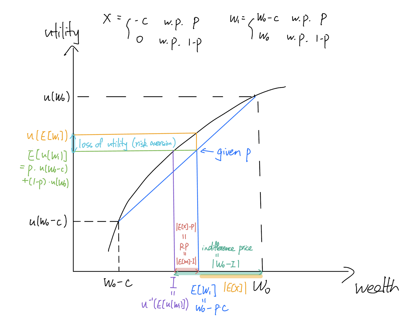
Certainty equivalent
- Denote the initial situation as \(A\). We have \[ E[u(A)] = p u(W_0-c) + (1-p) u(W_0).\]
- Denote now situation \(B\), whereby Hugo has wealth \(I\) with certainty. We have \[ E[u(B)] = u(I).\]
- We call \(I\) the “certainty equivalent” to \(A\) if \[A \sim B \Longleftrightarrow E[u(A)] = E[u(B)] \Longleftrightarrow I = u^{-1}(E[u(A)]).\]
General case
- Assume now that the loss is no longer as simple as \(c\) with probability \(p\), but a more general random variable $ \(X \in \mathbb{R}\).
- The certainty equivalent is \[I = u^{-1} \left( \; E\left[ u(W_0+X)\right]\; \right).\]
- The indifference price is \[ P = I - W_0.\]
- The risk premium is \[\text{risk premium} = E[X]-P.\] This is the maximum amount an insurer would be able to charge for full protection against \(X\), if the DM faced with \(X\) has utility function \(u(\cdot)\), and if the DM follows the EUT.
Examples
Umbrellas vs Ice cream
The certainty equivalent for each option is \[ (\gamma \cdot E[u(W_0+X)]+1)^{1/\gamma},\] that is, noting that the numbers in the table ore of the type “\(u(W_0+X)\)”, we get
- $7,414 for umbrellas, and
- $7,661 for ice creams.
This means that (according to this utility function)
- Ella would be better off keeping her savings ( \(W_0\) ) if they exceed those amounts (if \(W_0>I\));
- Ella should be prepared to pay $247 more for the ice cream project than for the umbrella one.
St Petersburg paradox
The certainty equivalent of $ \(X\) here is \[ \exp\{ E[u(X)]\} = \exp\{ 2 \log 2\} = 4.\]
This means that an individual with log utility and no money at all (here \(W_0=0\) would be indifferent between receiving $4 with certainty, and playing the game.
The result would be different in general depending on the initial amount of wealth of the individual.
Characterising risk aversion
Introduction
Umbrellas vs Ice creams: What if Ella’s wealth changes?
Assume now that Ella’s savings were $100,000, plus the cost of either projects. The table of utilities becomes
(computed using $100,000 plus profit for each case)
| Weather | Umbrellas | Ice creams | Probability |
|---|---|---|---|
| Bad | 719.1 | 636.7 | 1/4 |
| OK | 643.0 | 655.3 | 1/2 |
| Sunny | 636.7 | 679.2 | 1/4 |
| Expectation | 660.5 | 656.7 |
- We are back to preferring Umbrellas!
- That is because Ella has sufficient wealth to accept the much higher level of risk of Umbrellas. This extra risk no longer trumps the
extra level of expected profit.
Umbrellas vs Ice creams: What if \(\gamma\) changes?
Setting up functions in R:
power <- function(x,gamma){ (x^gamma-1)/gamma }

umbrella <- function(gamma,w0){
    expectedutility <- (power(w0+30000,gamma) + 2*power(w0+4000,gamma) + power(w0+2000,gamma))/4
    return( (expectedutility*gamma+1)^(1/gamma) ) }

icecream <- function(gamma,w0){
    expectedutility <- (power(w0+2000,gamma) + 2*power(w0+8000,gamma) + power(w0+16000,gamma))/4
    return( (expectedutility*gamma+1)^(1/gamma) ) }
Case 1: no wealth
Plot R code (result on the next slide):
par(cex=1.4)
curve(umbrella(x,0), from=0.01, to=0.99,
      lwd=2, col="blue",
      xlab="Parameter gamma (the smaller the more risk averse)",
      ylab="Certainty equivalent")
curve(icecream(x,0), from=0.01, to=0.99,
      add=TRUE, lwd=2, col="red")
abline(v=0.5849920142672, col="green")
text(0.6,6000, paste(signif(0.5849920142672, digits=3), sep=""),
     col="green", adj=0)
text(0.6,7600,"Ice cream", col="red", adj=0)
text(0.78,9000,"Umbrellas", col="blue", adj=1)
[Note R codes are not assessable!]

Case 2: wealth of 100,000
Plot R code (result on the next slide):
par(cex=1.4)
curve(umbrella(x, 100000) - icecream(x, 100000), from=0.01, to=0.99,
      lwd=2, col="black",
      xlab="Parameter gamma (the smaller the more risk averse)",
      ylab="Additional certainty equivalent of umbrellas")
abline(v=0.5849920142672, col="green")
[Note R codes are not assessable!]

Discussion
Observations:
- We have seen above that results in the Umbrella vs Ice cream example depend on the level of wealth, and also on the parameter of the utility function.
- More generally, results will depend on the shape of the utility function, and the region around which decisions are made (level of wealth \(W_0\)).
- When referring to “results” here, we refer to the attitudes of the decision maker towards risk, or “risk aversion”.
Is there a way of characterising risk aversion, that takes into account the utility assumptions and wealth, which we can use for comparisons?
(akin to mean and variance for location and spread of a distribution, for instance)
Absolute Risk Aversion
Definition
- Risk aversion means that we have a concave utility function.
- Concavity is equivalent to the fact that the DM has decreasing marginal utility from more wealth as they become richer: \(u'\), which is positive, becomes less and less positive as wealth increases: \(u''<0\).
- The more concave, the higher the risk premium (look back at the graph for the intuition).
- So a good first approximation for an (absolute) risk aversion ratio would be to look at \(u''\), standardised with \(u'\), say with a negative sign to make it positive for convenience.
- It turns out to be exactly that! The Absolute Risk Aversion (“ARA”) of wealth \(W\) is defined as \[ A(W) = - \frac{u''(W)}{u'(W)}.\]
- This is further “brought to life” in the next section
Examples:
- log utility \(u(w)=\log w\): we have \[u'(w) = \frac{1}{w} \text{ and } u''(w) = -\frac{1}{w^2}\] and hence \[A(w) = \frac{1}{w},\] which is directly inversely proportional to wealth.
- exponential utility \(u(w)=1-e^{-aw}\) ( \(a>0\) ): we have \[u'(w)=a e^{-aw} \text{ and }u''(w)=-a^2 e^{-aW}\] so that \[A(w) = a,\] which is constant, and provides a nice interpretation for
parameter \(a\) in the case of exponential utility.
Interpretation: risk premia via Taylor’s expansion
- A DM with utility function \(u\) has initial wealth \(W_0\) and faces risk \(X\).
- We have, by Taylor’s expansion (of \(u\) around \(W_0\)), that \[u(W_0+X) \approx u(W_0) + u'(W_0) X + \frac{1}{2}u''(W_0) X^2.\] Assume (w.l.o.g.) that \(E[X]=0\) and hence that \(Var(X)=E[X^2]\equiv \sigma^2\), which implies that (plugging those above) \[E[u(W_0+X)] \approx u(W_0) + \frac{1}{2} u''(W_0)\sigma^2.\]
- Separately, also by Taylor’s expansions, \[u(I)=u(W_0+P)\approx u(W_0) + u'(W_0) P.\]
- By definition, \[u(I) = E[u(W_0+X)],\] and hence \[\frac{1}{2} u''(W_0)\sigma^2 \approx u'(W_0) P \Longleftrightarrow P \approx \frac{1}{2}\frac{u''(W_0)}{u'(W_0)} \sigma^2 = - \frac{A(W_0)}{2} \sigma^2.\] This shows that the indifference price is (approximately) proportional to the absolute risk aversion, which makes a lot of sense.
- Here the risk premium is \(-P\) (remember \(E[X]=0\) ), which means that it is simply \(A(W_0)\) scaled up by \(\frac{\sigma^2}{2}\).
Effect of wealth on ARA
- The formula for the ARA \(A(w)\) is a function of \(w\)
- This means that the ARA varies for different of wealth, which makes sense: a millionaire is more likely gamble $100 than a poor student with no money.
- In general, one expects the ARA to be decreasing with wealth, that is, \[A'(w) < 0.\]
- If, on the other hand \(A'(w)=0\), this means that the risk premium is constant for any levels of wealth.
- Examples:
- log utility: \(A'(w) = - w^{-2} < 0\).
- exponential utility: \(A'(w) = 0\). Here the risk premium is insensitive to wealth.
Relative Risk Aversion
Think in relative terms
- Think now in relative terms.
- Rather than “adding” random \(X\) to \(W_0\), we multiply \(W_0\) by a random factor \(Z\) with \(E[Z]=1\) and \(Var(Z)=E[Z^2]-1\equiv \sigma^2\).
- So our wealth after risk has been applied is \(W_0\cdot Z\).
- We must now define the certainty equivalent as \[ u(I) = E[u(W_0\cdot Z)].\]
- The indifference price should also be defined in relative terms, that is, \[I-W_0 \equiv - \pi_R W_0\text{ so that } \pi_R=\frac{W_0-I}{W_0}.\]
Help via Taylor’s expansion
- Let’s expand \(u(W_0 Z)\) around \(W_0\).
- Noting that \[W_0 Z-W_0= W_0 (Z-1),\] which as mean 0 and variance \(W_0^2 \sigma^2\), we get \[u(W_0 Z) \approx u(W_0)+u'(W_0) (W_0 Z-W_0) + u''(W_0)\frac{(W_0 Z-W_0)^2}{2},\] and hence that \[E[u(W_0 Z)] \approx u(W_0) + \frac{1}{2} \sigma^2 u''(W_0) W_0^2.\]
- Similarly, noting that \[I = W_0 - \pi_R W_0,\] we get (via Taylor) that \[u(I) \approx u(W_0) - \pi_R u'(W_0) W_0.\]
- Combining those two results as before yields \[\pi_R = -\frac{\sigma^2}{2}W_0 \frac{u''(W_0)}{u'(W_0)}.\]
This result is analogous to the one we had for the ARA, but in relative terms. This leads to the definition in the next slide.
Definition
The Relative Risk Aversion (“RRA”) for a DM with utility function \(u\) is defined as \[R(w) = -w\frac{u''(w)}{u'(w)}.\]
Examples:
- log utility: \[R(w) = wA(w) = 1.\] In this case, the log utility is the one with constant RRA. The DM only cares about the proportion of their wealth they will lose, irrespective of their wealth level.
- exponential utility: \[R(w) = wA(w) = aw,\] which increases with wealth. In this case, the DM realises that a constant proportion of a larger amount of money is more money,
and so their wealth will impact their RRA.
Additional considerations
How do you come up with a utility function?
There are essentially two different types of use:
- “Assume” a utility function, which we believe is appropriate to the context, to draw insights from a stylised theoretical model.
- For instance, one might ask what the optimal way of investing money in retirement is (a hot topic!).
- As an example, see
the published paper coming out of Lewis de Felice's 2023 honours essay
- Gather data (choices) about an individual, and try to “fit” an appropriate utility function to those choices.
- The result could be informative in itself (such as in supporting assumptions such as those made in the previous case), and/or
- could be used to support decision making.
When one function is not enough
- There is no guarantee that a single utility function will fit well:
- for all wealth levels: we may need to paste different functions for different areas;
- in all circumstances: the risk aversion of the DM may be affected by some “state” (e.g., being married vs widowed, or healthy vs sick, for a retiree).
- Hence, there may be circumstances where state-dependent, and/or pasted utility functions may be warranted.
Limitations to the EUT
- The EUT was gigantic step forward towards being able to describe decision making of humans.
- It suffers from a number of flaws and limitations, though. Here are a few:
- It assumes we can determine someone’s utility function, which is a strong assumption.
- It requires being able to describe risk with certainty. In reality there is uncertainty about outcomes, which complicates things.
- Whether a company has a utility function is debatable (and debated!). At best, it makes decision on the basis of a combination of different utility functions (the decision makers). In the worst case, it is simply impossible to describe decision making with a utility function. One can also argue that risk aversion is a trait of human nature, which is not relevant to a company.
Alternatives to describing behaviour
There are many refinements and alternatives to the EUT, to support/describe decision-making. The ones mentioned in the syllabus (and taught in ACTL30006) are
- mean-variance portfolio theory (see Joshi (2013)) — this is very similar to using a quadratic utility function;
- behavioural finance (Section 3 of IoA 2023).
This is a whole (fascinating) field in itself, but we need to stop here for now!
References
Selected references:
IoA. 2023. Course Notes and Core Reading for Subject CM2 Models. The Institute of Actuaries.
Joshi, Mark Suresh. 2013. Introduction to Mathematical Portfolio Theory. Cambridge University Press.