M2 Basic Reserving Concepts

Topics in Insurance, Risk, and Finance

Introduction - Claims liabilities

Definition

• Generally in insurance, premiums are collected first, before coverage is provided. The insurer can’t consider this premium as income before coverage is provided.
• Furthermore, as times goes by, the insurer does not know instantly how much losses it will have to pay (e.g., delays in notification, delays in payments).

---

• This gives rise to two types of liabilities:
  • Unearned premium liability: an amount set aside for covering losses related to coverage not yet provided, but where a premium has already been collected;
  • Outstanding claim liability: an amount set aside for for covering losses corresponding to coverage that has already been provided, but where payments are still expected to occur.
• These take a significant proportion of an insurer’s balance sheet, often multiple times its equity, as exemplified in the IAG example (forthwith).
• It is the actuary’s responsibility to determine those amounts

It’s a huge responsibility!

The case of IAG

Insurance Australia Group is one of the largest Australian general insurers (the largest under some measures). Its latest Balance Sheet (as at 31 December 2024, see page 22 of the financial report) shows:

• Assets
  • Total: 24,956m (100%)
• Liabilities
  • Insurance contract liabilities: 14,139m (56.7%), of which (p. 33)
    • Liability for remaining coverage: 2,191m (8.8%)
    • Liability for incurred claims: 11,948 (47.9%)
  • Other: 3,783m (15.1%)
• Equity
  • Total: 7,034 (28.2%)

It is worth noting that IAG holds 2.07 times the APRA “Prescribed Capital Amount” (PCA), see page 7. See https://www.iag.com.au/results-and-reports to download the latest financial statements of IAG.

The claims process

Main reference

Note that figures, notation, examples and structure are mostly drawn from Taylor (2000), which is the main reference for Modules 2–5.

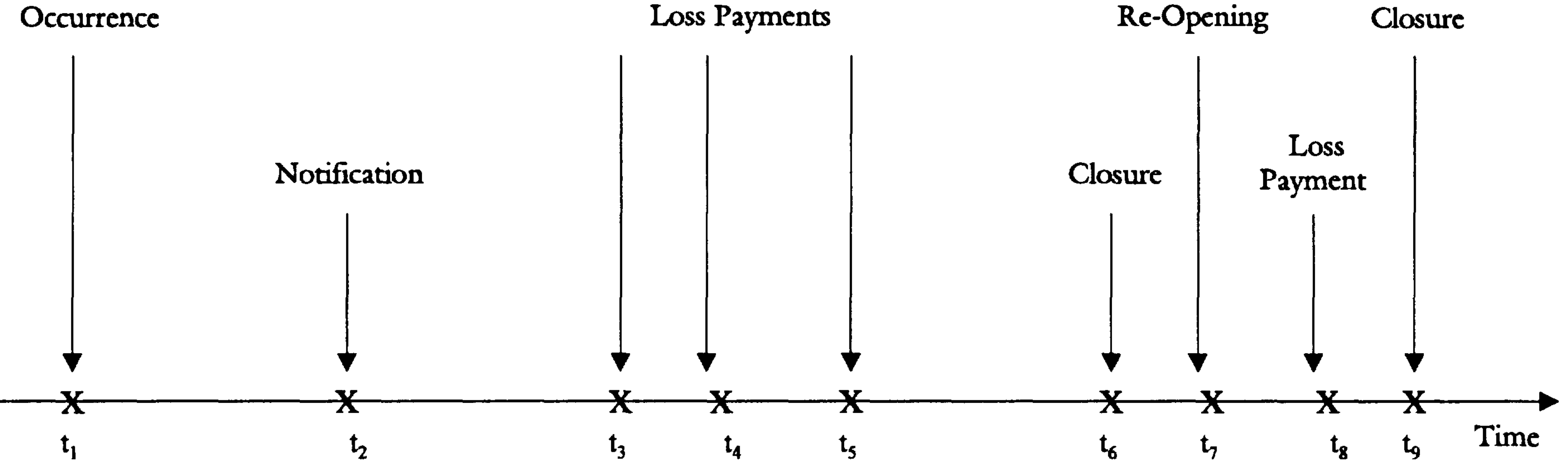
Time line of a claim and IBNR

From $t_1$ to $t_2$:

• A liability exists (an insured event occurred)
• However, the insurer is unaware of the claim
• During this interval, the claim is said to be incurred but not reported (or “IBNR”).

---

From $t_2$ and $t_9$:

• There will be future payments, even though the insurer may not know with certainty about them
• These should be captured by an appropriate reserve.

Inflation

• Because claims are paid at different points in time, they are subject to inflation.
• Inflation will generally be different from CPI, and is typically specific to a line of business. Let $\lambda (t)$ be an index describing such claims inflation.
• Inflation may continue beyond the point of occurrence of a claim, up to the point of payment.
  • This can have a very long duration (e.g. income in workers compensation)

---

We define: $$C^{\ast }=\sum _{j=3,4,5,8}C(t_j)$$ as the sum of payments $C(t_j)$ all expressed in dollars as of $t_1$ (date of occurrence), and $$C=\sum _{j=3,4,5,8}C(t_j)\frac{\lambda (t_j)}{\lambda (t_1)},$$ as the sum of the nominal (actual) amounts paid.

(Note that superimposed inflation - Section 1.1.4 - is not in scope this year)

Estimates of outstanding loss liability

General

Now assume that an evalutaion of liability is required at time $t$:

---

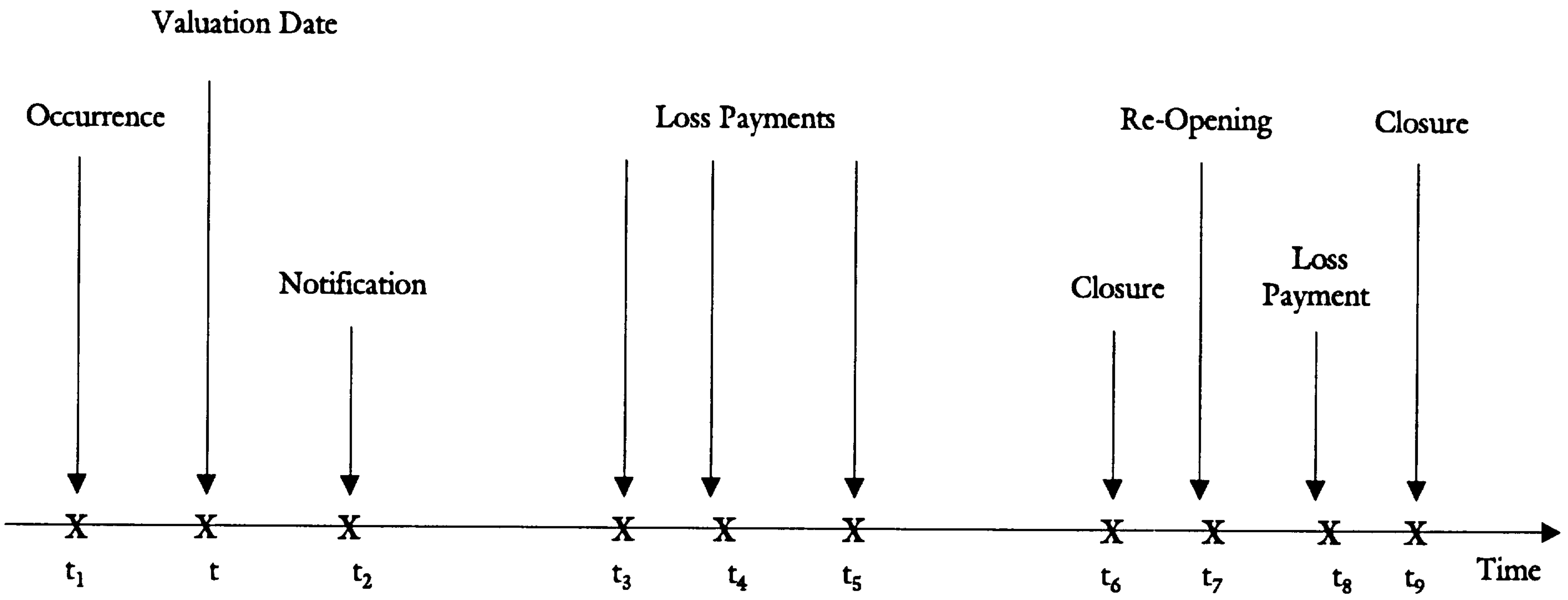
Note

• if $t\ge t_1$: the liability exists, and ideally the claim should be considered in some shape or form.
• if $t_1\ge t\ge t_2$: claim is unknown, but the insurer knows that there are unknowns. It will try to estimate those as “IBNR” (see also next module).
• if $t\ge t_2$: claim will be known, and the insurer will try to estimate its cost (case reserve).
• between $t_6$ and $t_7$, as well as after $t_9$, the insurer’s estimate will be zero (because the claim is deemed closed).

Time dimensions of “periods”

Let:

• a $period$ be some appropriate measure of time length, such as a month, quarter or year.

Now when referring to a specific claim payment, it can be classified according to:

• $i$ being the period of origin where $i=0,\dots ,I$
  • this is the period when the claim occurred (in most cases) or reported (in the rare case of “claims-made” policies)
• $j$ being the development period where $j=0,\dots$
  • this is difference in period index between occurrence and payment (0 if the payment happens in the same period as occurrence)
• $k=i+j$ being the calendar period where $k=0,\dots$
  • $k=0$ is the earliest period with data
  • also called experience period

---

This illustrates those concepts:

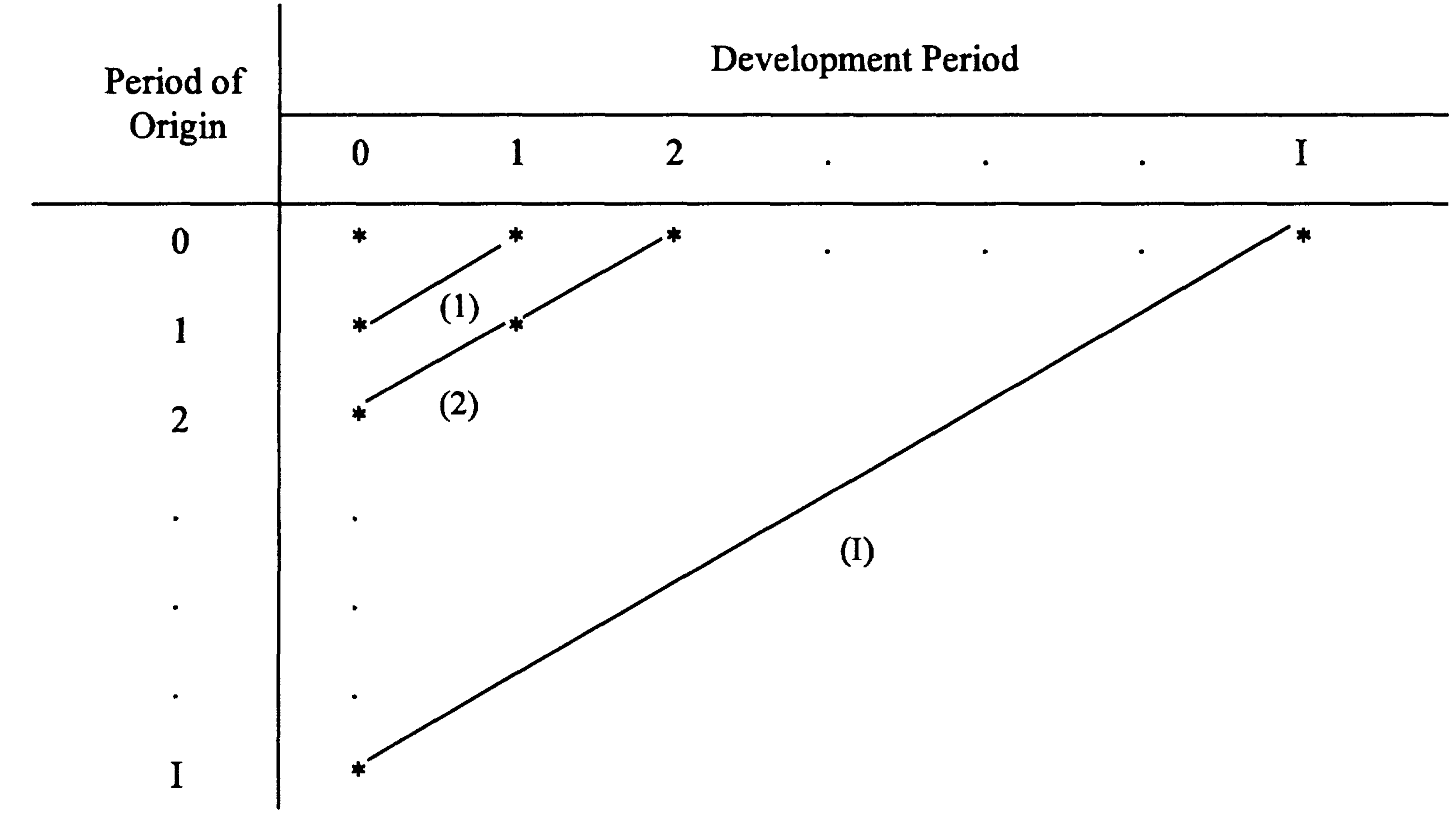
Relation between periods of origin, development and experience.

Further notation

• $C(i,j)$: paid losses in the $(i,j)$ cell
• Outstanding loss liability at the end of $j$ (or $k$) for $i$: $$P(i,j)\equiv \bar{P}(i,k)\equiv \sum _{m=j+1}^{\mathrm{\infty }}C(i,m)$$ (note you can replace $j$ with $k-i$ in the lower bound)
• Total outstanding loss liability at the end of $k$ - for all periods of origin: $$\bar{P}(k)=\sum _{i=0}^I\bar{P}(i,k)=\sum _{i=0}^I\sum _{m=k-i+1}^{\mathrm{\infty }}C(i,m).$$
• Both $\bar{P}(i,k)$ and $\bar{P}(k)$ are aggregate amounts (not claims based).
• While the textbook says that most actuarial estimates are aggregate, individual claims reserving has gathered a lot of momentum
  since then, thanks to data availability, computing power
  and machine learning capabilities.

Components of outstanding loss liability

Cash flows

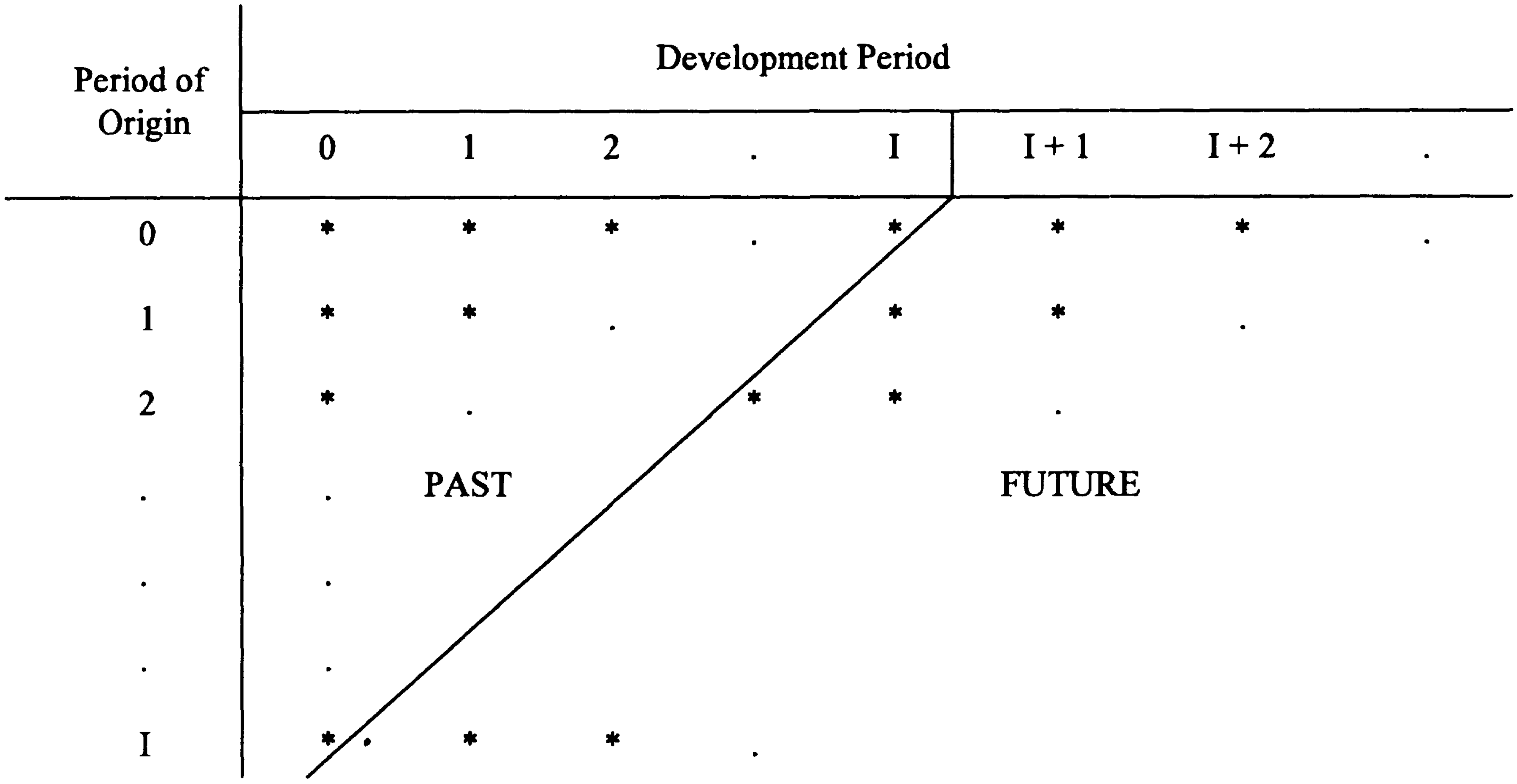
The equation above is about “completing the rectangle”,
as illustrated above.

Claims inflation

Usually, the reserving technique will yield estimates of $C^{\ast }$, that is, as of dollars of some base date (usually current date), so that $$C(i,j)=C^{\ast }(i,j)\frac{\lambda (k)}{{\lambda }_0},$$ where

• $\lambda (k)$ is the relevant claims inflation index;
• ${\lambda }_0$ is the value of that index on the base date.

(again, superimposed inflation is out of scope, but can conceptually be seen as adjusting $\lambda$ appropriately)

Loss adjustment expenses

We consider:

• allocated loss adjustment expenses (ALAE)
  • These can be linked to specific claims.
  • These are typically included in the $C(i,j)$ and don’t require extra treatment.
• unallocated loss adjustment expenses (ULAE)
  • These cannot be easily linked to specific claims (think overhead costs, for instance).
  • These are typically not in the $C(i,j)$ and will require specific consideration if they are to be included.
  • Denote $$e(i,j)$$ as the proportion of paid losses to be added to costs for ULAE.

Investment income

• Liabilities will have assets covering them on the balance sheet.
• These may be invested, and it may be required to consider corresponding investment returns.
• That is, if the $10 you have to pay in 5 years can be covered with $9 today (even after allowing for inflation), then you may be required/allowed to reserve $9 instead of $10.
• Let $d(k)$, $k=I+1,I+2,\dots$, be the discount factor to be applied for payments made in experience period $k$ (in the example above, we would have $d(I+5)=9/10$) .
• Note that $\lambda \ne d$: there is no reason why claims inflation should evolve in the same identical way to your investments.

---

In the end, we have:

$$\begin{array}{rcl}\bar{P}(k)& =& \sum _{i=0}^I\sum _{m=k-i+1}^{\mathrm{\infty }}C(i,m)[1+e(i,m)]d(i+m)\\ & =& \sum _{i=0}^I\sum _{m=k-i+1}^{\mathrm{\infty }}{C}^{\ast }(i,m)\frac{\lambda (i+m)}{{\lambda }_0}[1+e(i,m)]d(i+m).\end{array}$$

Recoveries

Possible recoveries (offsetting claims):

• reinsurer payments;
• third parties at fault;
• salvage value (for property insurance).

Generally speaking, insurers have a subrogation right, which allows them to seek compensation on behalf of the insured if they believe it is worth the effort.

This can be considered as negative $C(i,j)$, or may require another triangle altogether. Specific treatment is outside scope here.

Loss reserving

General

• So far, we have defined the “oustanding loss liability” as a random variable - this is the actual amount that will have to be paid.
• In general this is unknown, and now the question is how to estimate this, and how much to set aside for covering those liabilities.
• It makes sense that you would reserve its expectation plus some margin, so that we define:
  • Expected outstanding loss liability: this is the expectation, also called central estimate;
  • Prudential margin or risk margin: this is the margin you add to the central estimate to allow for estimation error, and “worse than average” cases.
• In the end we have: $$\text{loss reserve }=\text{ central estimate }+\text{ risk margin}.$$

In Australia

Legislative framework

The Standard governing actuarial valuations of insurance liabilities is found at www.legislation.gov.au

• Section 8 states that “An insurer must determine a value for both its outstanding claims liabilities and its premiums liabilities for each class of business underwritten by the insurer.”
• Sections 9 defines “outstanding claims liabilities” as relating “to all claims incurred prior to the valuation date, whether or not they have been reported to the insurer”.
• Section 10 defines “premium liability” as relating “to all future claim payments arising from future events post the valuation date that will be insured under the insurer’s existing policies that have not yet expired”.

Outstanding claims liability in Australia

APRA’s GRS 210 (where "RS" stands for "Reporting standards") says:

The valuation of outstanding claims liabilities for each class of business must comprise:

1. a central estimate (refer below); and
2. a risk margin (refer below) that relates to the inherent uncertainty in the central estimate values.

---

Furthermore, it continues on by clarifying:

The valuation of insurance liabilities (i.e. outstanding claims liabilities and premiums liabilities) reflects the individual circumstances of the Level 2 insurance group. In any event, the value of insurance liabilities must be the greater of a value that is:

1. determined on a basis that is intended to value the insurance liabilities of the Level 2 insurance group at a 75 percent level of sufficiency; and
2. the central estimate plus one half of a standard deviation above the mean for the insurance liabilities of the Level 2 insurance group.

There’s a lot more information in the document.

Solvency capital requirements in Australia

• Additionally, solvency requirements (look for “GPS”, where “PS” stands for “Prudential Standards”) require insurers to hold capital corresponding (typically) to a 99.5-ile at the company’s level (including diversification benefits), which requires knowledge of the distribution of future payments quite far in the tail, and how they interact across lines of business.
• This is similar in Europe with Solvency II.
• Of course, it is a little more complicated than that, but the main point is that you might need to work out the distribution of payments quite far in the tail.

Data

Nature

Generally, available data includes at least:

• claim counts (open / closed);
• claim payments;
• case estimates.

Nowadays, one also typically has:

• details of payment dates for each claim;
• details of case reserve amounts and associate revision dates for each claim;
• additional data such as policy data, claims qualitative data (description of the event), etc…

These can be (are nowadays increasingly) used for improving reserving, but this is outside scope of this subject.

Aggregate data

Incremental data

In the case of aggregate data, each cell $(i,j)$ will have data of four types:

• $N(i,j)$ are the counts of claims notified;
• $C(i,j)$ are paid losses;
• $U(i,j)$ are the counts of claims open ;
• $Q(i,j)$ are the case estimates of outstanding liability.

Because those numbers refer to cell $(i,j)$ only, we often refer to the as incremental data.

Cumulative data

It is sometimes convenient to express data in cumulative terms.

We define: $$A(i,j)=\sum _{m=0}^{j}N(i,m)$$ as cumulative counts data, with $$N(i)=A(i,\mathrm{\infty })$$ being the ultimate count of incurred claims.

---

Payment data can be similarly accumulated: $$D(i,j)=\sum _{m=0}^{j}C(i,m)$$ such that $$I(i,j)=D(i,j)+Q(i,j)$$ are the estimated amounts of incurred losses (note that even if this is indexed $(i,j)$ it is of cumulative nature).

References

Selected references:

Taylor, Greg. 2000. Loss Reserving: An Actuarial Perspective. Huebner International Series on Risk, Insurance and Economic Security. Kluwer Academic Publishers.